But Excel starts to get very powerful when you use formulas to compare data and create new information. Excel supports a large number of formulas that can add, subtract, multiply, divide and compare data, so it is beneficial to learn the basics of Excel formulas so that you can begin using them to your advantage. Our tutorial below will show you how to create a simple multiplication formula in a cell, then copy and paste it into other cells in the same column. We will then direct you to the Formulas menu where you can select new formulas that you want to use.
Creating Formulas in an Excel 2013 Worksheet
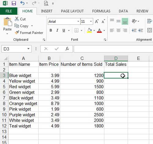
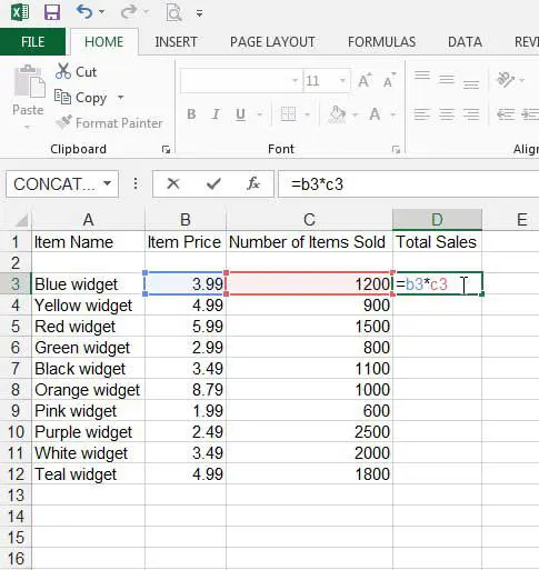
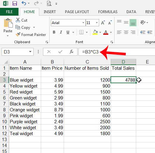
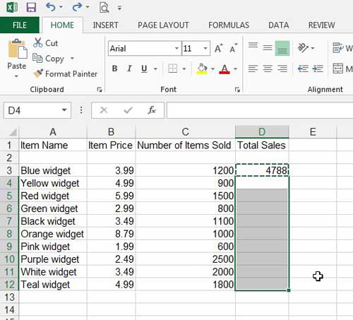
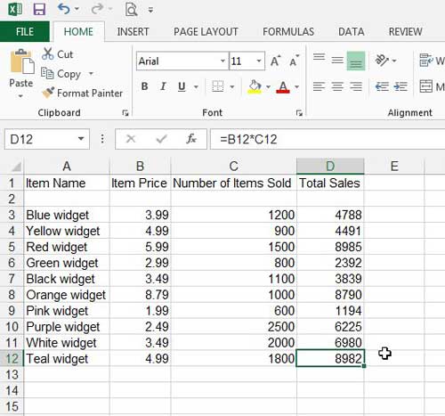
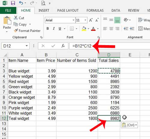
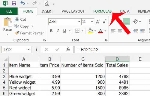
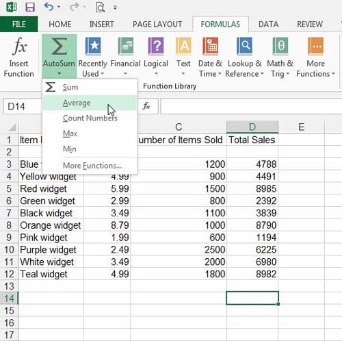
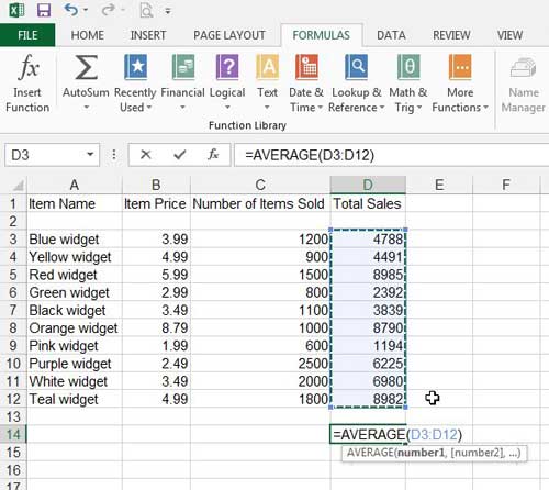
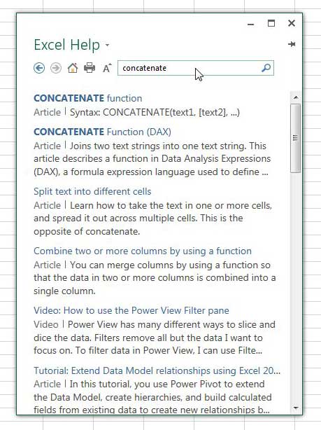
This tutorial is going to teach you how to manually type a formula into a cell in Excel 2013 that multiplies a value in one cell by a value in another cell. We will then copy that formula into the rest of the cells in the column, where the formula will update to include the values for the cells in the new row. This allows you to quickly apply the same formula to all of the values in your columns without needing to manually retype the formula. Step 1: Open your worksheet in Excel 2013. Step 2: Click inside the cell where you want the result from your formula to be displayed. Step 3: Type the formula =XXYY where XX is the first cell containing a value that you want to multiply and YY is the second value that you want to multiply. Press Enter on your keyboard to execute the formula. You have now used a formula to produce new data from your information. We will continue below to learn how to apply this formula to other cells. Step 4: Click on the cell containing your formula answer, then press Ctrl + C on your keyboard to copy it. Note that the value is displayed in the cell, but that you can see the formula in the Formula Bar above the worksheet. Step 5: Highlight the cells underneath your formula into which you want to copy this formula. The result should look like the image below. Step 6: Press Ctrl + V on your keyboard to fill the selected cells with the formula that you copied in Step 4. You will note that Excel has automatically updated the values in your formula so that they are relative to your original formula. For example, if I click on the bottom cell of the range that I selected in Step 5, you can see that the formula has updated so that it is multiplying cells B12C12 instead of cells B3*C3. You can find additional formulas by clicking the Formulas tab at the top of the window. For example, if I wanted to find the average of the values that I just calculated with my multiplication formula, I could click inside a cell where I wanted to display the average, then select the Average formula. I can then use my mouse to select the cells for which I want to find the average, then press Enter on my keyboard to calculate it. Excel has a huge selection of formulas that you can use, many of which can save you a lot of time. Take some time to look around and experiment with some of these functions to see what they can do. If you have questions about a formula, you can always click the Help icon (the ? icon) at the top-right corner of the window and type the name of the function into the search field to learn more about it. Do you need more or fewer decimal places in your cells? Learn how to adjust the number of decimal places with this article. After receiving his Bachelor’s and Master’s degrees in Computer Science he spent several years working in IT management for small businesses. However, he now works full time writing content online and creating websites. His main writing topics include iPhones, Microsoft Office, Google Apps, Android, and Photoshop, but he has also written about many other tech topics as well. Read his full bio here.
You may opt out at any time. Read our Privacy Policy
