While labeling columns with headers or titles can be helpful, you can really improve your accuracy by freezing the top row that contains that information. This will keep the top row locked to the top of the spreadsheet so that it remains visible while you are scrolling down. Our tutorial below will show you how to freeze a row in Google Sheets.
Always Show the Top Row of a Spreadsheet in Google Sheets
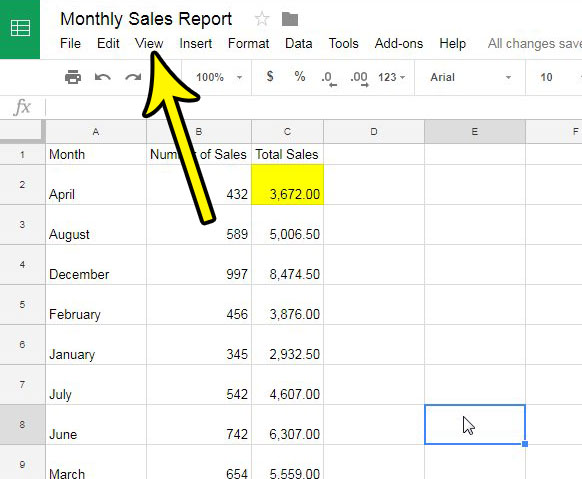
The steps in this article were performed in Google Chrome, but will also work in other Web browsers like Firefox and Internet Explorer. Note that this setting only applies to the current spreadsheet. It will not affect the display of any other spreadsheets in your Google Drive. Step 1: Go to your Google Drive at https://drive.google.com/drive/my-drive and open the Sheets file with the top row that you wish to freeze. Step 2: Click the View tab at the top of the window.
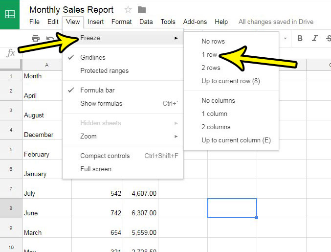
Step 3: Select the Freeze menu item, then click on the 1 row option.
Note that there are several other options for freezing columns and rows on this menu as well, if you are looking to freeze some data, but not necessarily the top row. Do you need to add another column of data in your spreadsheet, but you want to put it between two existing columns? Find out how to insert a column in Google Sheets and avoid the need to manually cut and paste your data. He specializes in writing content about iPhones, Android devices, Microsoft Office, and many other popular applications and devices. Read his full bio here.


